Quickstart

Here are some quickstart examples making use of the example data that comes with anesthetic and can be found in anesthetic’s test folder.

Plotting marginalised posteriors

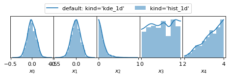
Plot Example 1: Marginalised 1D posteriors

from anesthetic import read_chains, make_1d_axes
samples = read_chains("../../tests/example_data/pc")
params = ['x0', 'x1', 'x2', 'x3', 'x4']
fig, axes = make_1d_axes(params, figsize=(6, 1.8), facecolor='w', ncol=5)
samples.plot_1d(axes, label="default: kind='kde_1d'")
samples.plot_1d(axes, kind='hist_1d', color='C0', alpha=0.5, zorder=0, label="kind='hist_1d'")
axes['x0'].legend(bbox_to_anchor=(2.5, 1), loc='lower center', ncol=2)

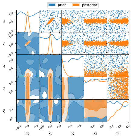
Plot Example 2: Marginalised 2D posteriors

from anesthetic import read_chains, make_2d_axes
samples = read_chains("../../tests/example_data/pc_250")
prior = samples.prior()
params = ['x0', 'x1', 'x2', 'x3', 'x4']
fig, axes = make_2d_axes(params, figsize=(6, 6), facecolor='w')
prior.plot_2d(axes, alpha=0.9, label="prior")
samples.plot_2d(axes, alpha=0.9, label="posterior")
axes.iloc[-1, 0].legend(bbox_to_anchor=(len(axes)/2, len(axes)), loc='lower center', ncols=2)

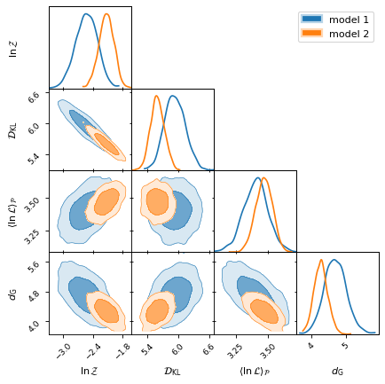
Nested sampling statistics

Providing Bayesian statistics from nested sampling data is where anesthetic shines. With anesthetic.samples.NestedSamples.stats() you can compute the Bayesian evidence \(\ln\mathcal{Z}\), the Kullback–Leibler divergence \(\mathcal{D}_\mathrm{KL}\), and the posterior average of the log-likelihood \(\langle\ln\mathcal{L}\rangle_\mathcal{P}\), which together allow you to jointly assess model quality, Occam penalty, and fit, respectively. The Gaussian model dimensionality \(d_\mathrm{G}\) (which is directly related to the posterior variance of the log-likelihood) is a measure of the model complexity (or dimensionality).

from anesthetic import read_chains, make_2d_axes
samples1 = read_chains("../../tests/example_data/pc")
samples2 = read_chains("../../tests/example_data/pc_250")
stats1 = samples1.stats(nsamples=2000)
stats2 = samples2.stats(nsamples=2000)
params = ['logZ', 'D_KL', 'logL_P', 'd_G']
fig, axes = make_2d_axes(params, figsize=(6, 6), facecolor='w', upper=False)
stats1.plot_2d(axes, label="model 1")
stats2.plot_2d(axes, label="model 2")
axes.iloc[-1, 0].legend(bbox_to_anchor=(len(axes), len(axes)), loc='upper right')