Weighted samples: the `Samples`, `MCMCSamples`, and `NestedSamples` data frames

The anesthetic.samples.Samples data frame at its core is a pandas.DataFrame, and as such comes with all the pandas functionality. The anesthetic.samples.MCMCSamples and anesthetic.samples.NestedSamples data frames share all the functionality of the more general Samples class, but come with some additional MCMC or nested sampling specific functionality.

from anesthetic import read_chains, make_2d_axes
samples = read_chains("../../tests/example_data/pc_250")

General weighted sample functionality

The important extension to the pandas.Series and pandas.DataFrame classes, is that in anesthetic the data frames are weighted (see anesthetic.weighted_pandas.WeightedSeries and anesthetic.weighted_pandas.WeightedDataFrame), where the weights form part of a pandas.MultiIndex and are therefore retained when slicing.

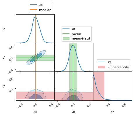
Mean, standard deviation, median, quantiles, etc.

The weights are automatically taken into account in summary statistics such as mean, variance, covariance, skewness, kurtosis, standard deviation, median, quantiles, etc.

x0_median = samples.x0.median()
x1_mean = samples.x1.mean()
x1_std = samples.x1.std()
x2_min = samples.x2.min()
x2_95percentile = samples.x2.quantile(q=0.95)

fig, axes = make_2d_axes(['x0', 'x1', 'x2'], upper=False)
samples.plot_2d(axes, label=None)
axes.axlines({'x0': x0_median}, c='C1', label="median")
axes.axlines({'x1': x1_mean}, c='C2', label="mean")
axes.axspans({'x1': (x1_mean-x1_std, x1_mean+x1_std)}, c='C2', alpha=0.3, label="mean+-std")
axes.axspans({'x2': (x2_min, x2_95percentile)}, c='C3', alpha=0.3, label="95 percentile")
axes.iloc[0, 0].legend(bbox_to_anchor=(1, 1), loc='lower right')
axes.iloc[1, 1].legend(bbox_to_anchor=(1, 1), loc='lower right')
axes.iloc[2, 2].legend(bbox_to_anchor=(1, 1), loc='lower right')

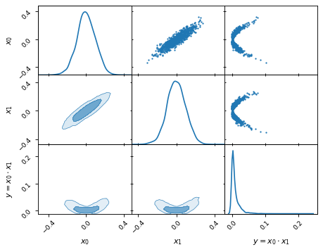
Creating new from existing columns

We can define new parameters with relative ease. For example, given two parameters x0 and x1, we can compute the derived parameter y = x0 * x1:

samples['y'] = samples['x1'] * samples['x0']
samples.set_label('y', '$y=x_0 \\cdot x_1$')
samples.plot_2d(['x0', 'x1', 'y'])

MCMC statistics

Markov Chain Monte Carlo (short MCMC) samples as the name states come from Markov chains, and as such come with some MCMC specific properties and potential issues, e.g. correlation of successive steps, a burn-in phase, or questions of convergence.

We have an example data set (at the relative path anesthetic/tests/example_data/ with the file root cb) that emphasizes potential MCMC issues. Note, while this was run with Cobaya, we had to actually put in some effort to make Cobaya produce such a bad burn-in stage. With its usual optimisation settings it normally produces much better results.

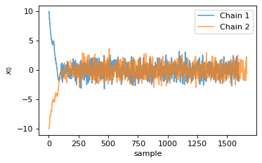
Chains

When MCMC data is read in, anesthetic automatically keeps track of multiple chains that were run in parallel via the 'chain' parameter. You can split the chains into separate samples via the pandas.DataFrame.groupby() method:

from anesthetic import read_chains, make_2d_axes
mcmc_samples = read_chains("../../tests/example_data/cb")
chains = mcmc_samples.groupby(('chain', '$n_\\mathrm{chain}$'), group_keys=False)
chain1 = chains.get_group(1)
chain2 = chains.get_group(2).reset_index(drop=True)

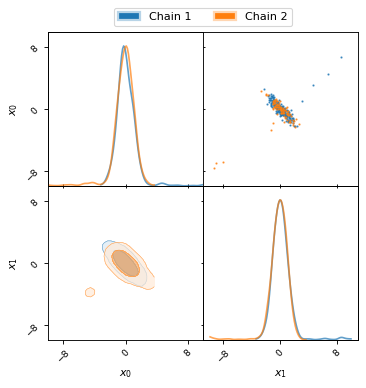
For this example MCMC run the initial burn-in phase is very apparent, as can be seen in the following two plots.

fig, ax = plt.subplots(figsize=(5, 3))
ax = chain1.x0.plot.line(alpha=0.7, label="Chain 1")
ax = chain2.x0.plot.line(alpha=0.7, label="Chain 2")
ax.set_ylabel(chain1.get_label('x0'))
ax.set_xlabel("sample")
ax.legend()

fig, axes = make_2d_axes(['x0', 'x1'], figsize=(5, 5))
chain1.plot_2d(axes, alpha=0.7, label="Chain 1")
chain2.plot_2d(axes, alpha=0.7, label="Chain 2")
axes.iloc[-1, 0].legend(bbox_to_anchor=(len(axes)/2, len(axes)), loc='lower center', ncol=2)

Remove burn-in

To get rid of the initial burn-in phase, you can use the anesthetic.samples.MCMCSamples.remove_burn_in() method:

mcmc_burnout = mcmc_samples.remove_burn_in(burn_in=0.1)

Positive burn_in values are interpreted as the first samples to remove, whereas negative burn_in values are interpreted as the last samples to keep. You can think of it in the usual python slicing mentality: samples[burn_in:].

If 0 < abs(burn_in) < 1 then it is interpreted as a fraction of the total number of samples in the respective chain.

To see how remove_burn_in has removed the burn-in samples in both chains, see the plot in the following section, alongside an assessment of convergence.

Gelman–Rubin statistic

Another important issue when it comes to MCMC samples is assessing convergence. In anesthetic we have implemented the modified Gelman–Rubin statistic as described in Antony Lewis (2013). For the underlying (more theoretical) accounts of this statistic, see e.g. Gelman and Rubin (1992) and Brooks and Gelman (1998).

Provided you have an MCMC run containing multiple chains, you can compute the Gelman–Rubin R-1 statistic using the anesthetic.samples.MCMCSamples.Gelman_Rubin() method:

Rminus1_old = mcmc_samples.Gelman_Rubin()
Rminus1_new = mcmc_burnout.Gelman_Rubin()
Rminus1_par = mcmc_burnout.Gelman_Rubin(per_param='par')

You can get the convergence per parameter by passing the keyword per_param='par'. By passing per_param='cov' you will even get the covariant part of the convergence of pairs of parameters.

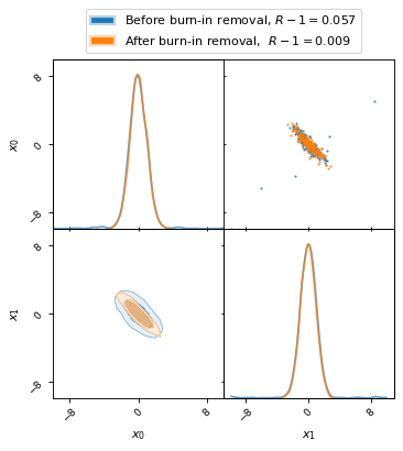
The following plot shows how remove_burn_in gets rid of burn-in samples. Note the stark difference in the Gelman–Rubin statistic, as listed in the legend, depending on whether burn-in samples were removed or not.

fig, axes = make_2d_axes(['x0', 'x1'], figsize=(5, 5))
mcmc_samples.plot_2d(axes, alpha=0.7, label="Before burn-in removal, $R-1=%.3f$" % Rminus1_old)
mcmc_burnout.plot_2d(axes, alpha=0.7, label="After burn-in removal,  $R-1=%.3f$" % Rminus1_new)
axes.iloc[-1, 0].legend(bbox_to_anchor=(len(axes)/2, len(axes)), loc='lower center')

Note

Unless you specify which parameters to compute the Gelman–Rubin statistic for (by passing the keyword params), anesthetic will use _all_ parameters in the data frame except those containing ‘prior’, ‘chi2’, or ‘logL’ in their name. So if you for example want to exclude derived parameters, you should pass params directly.

Nested sampling statistics

Anesthetic really comes to the fore for nested sampling (for details on nested sampling we recommend John Skilling, 2006). We can do all of the above and more with the power that nested sampling chains provide.

from anesthetic import read_chains, make_2d_axes
nested_samples = read_chains("../../tests/example_data/pc")
nested_samples['y'] = nested_samples['x1'] * nested_samples['x0']
nested_samples.set_label('y', '$y=x_0 \\cdot x_1$')

Prior distribution

While MCMC explores effectively only the posterior bulk, nested sampling explores the full parameter space, allowing us to calculate and plot not only the posterior distribution, but also the prior distribution, which you can get with the anesthetic.samples.NestedSamples.prior() method:

prior_samples = nested_samples.prior()

Note

Note that the .prior() method is really just a shorthand for .set_beta(beta=0), i.e. for setting the inverse temperature parameter beta=0 (where 1/beta=kT) in the anesthetic.samples.NestedSamples.set_beta() method, which allows you to get the distribution at any temperature.

This allows us to plot both prior and posterior distributions together. Note, how the prior is also computed for the derived parameter y:

fig, axes = make_2d_axes(['x0', 'x1', 'y'])
prior_samples.plot_2d(axes, label="prior")
nested_samples.plot_2d(axes, label="posterior")
axes.iloc[-1, 0].legend(bbox_to_anchor=(len(axes)/2, len(axes)), loc='lower center', ncol=2)

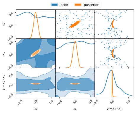
Note, how the uniform priors on the parameters x0 and x1 lead to a non-uniform prior on the derived parameter y.

Note further the different colour gradient in the posterior contours and the prior contours. While the iso-probability contour levels are defined by the amount of probability mass they contain, the colours are assigned according to the probability density in the contour. As such, the lower probability density in the posterior tails is reflected in the lighter colour shading of the second compared to the first contour level. In contrast, the uniform probability density of the prior distributions of x0 and x1 is reflected in the similar colour shading of both contour levels.

Bayesian statistics

Thanks to the power of nested sampling, we can compute Bayesian statistics from the nested samples, such as the following:

Bayesian (log-)evidence anesthetic.samples.NestedSamples.logZ()
Kullback–Leibler (KL) divergence anesthetic.samples.NestedSamples.D_KL()
Posterior average of the log-likelihood anesthetic.samples.NestedSamples.logL_P()
(this connects Bayesian evidence with KL-divergence as logZ = logL_P - D_KL, allowing the interpretation of the Bayesian evidence as a trade-off between model fit logL_P and Occam penalty D_KL, see also our paper Hergt, Handley, Hobson, and Lasenby (2021))
Gaussian model dimensionality anesthetic.samples.NestedSamples.d_G()
(for more, see our paper Handley and Lemos (2019))
All of the above in one go, using anesthetic.samples.NestedSamples.stats()

By default (i.e. without passing any additional keywords) the mean values for these quantities are computed:

bayesian_means = nested_samples.stats()

Passing an integer number nsamples will create a data frame of samples reflecting the underlying distributions of the Bayesian statistics:

nsamples = 2000
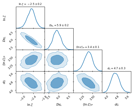
bayesian_stats = nested_samples.stats(nsamples)

Since bayesian_stats is an instance of anesthetic.samples.Samples, the same plotting functions can be used as for the posterior plots above. Plotting the 2D distributions allows us to inspect the correlation between the inferences:

fig, axes = make_2d_axes(['logZ', 'D_KL', 'logL_P', 'd_G'], upper=False)
bayesian_stats.plot_2d(axes);
for y, row in axes.iterrows():
    for x, ax in row.items():
        if x == y:
            ax.set_title("%s$ = %.2g \\pm %.1g$"
                         % (bayesian_stats.get_label(x),
                            bayesian_stats[x].mean(),
                            bayesian_stats[x].std()),
                         fontsize='small')

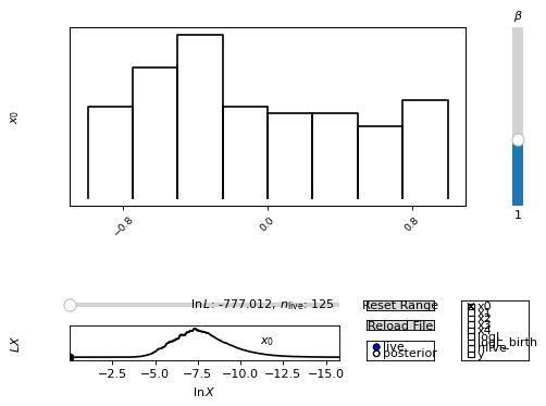
Nested Sampling GUI

We can also set up an interactive plot, which allows us to replay a nested sampling run after the fact.

nested_samples.gui()

Weighted samples: the Samples, MCMCSamples, and NestedSamples data frames